Implementation of GRASS GIS module for 3D raster flow line computation

Title:

Implementation of GRASS GIS module for 3D raster flow line computation

Student:

Anna Petrasova, ​North Carolina State University, Open Source Geospatial Research and Education Laboratory

Organization:

​OSGeo - Open Source Geospatial Foundation

Mentors:

​Helena Mitasova, ​Sören Gebbert

GSoC link:

​abstract

Abstract

GRASS GIS' capabilities of representing and processing data in 3D raster (voxel) format, are rare among other GIS software packages and open opportunities for new applications, especially in research. In this project I would like to extend the 3D raster handling capabilities by developing a module for computing 3D vector flow lines of a voxel representing trivariate continuous field. This new module, r3.flow, will extend the functionality of module r.flow into the third dimension.

Introduction

GRASS GIS' capabilities of representing and processing data in 3D raster (voxel) format, are rare among other GIS software packages and open opportunities for new applications, especially in research. In this project I would like to extend the 3D raster handling capabilities by developing a module for computing 3D vector flow lines of a voxel representing trivariate continuous field. This new module, r3.flow, will extend the functionality of module r.flow into the third dimension.

Background

Although GRASS GIS is mainly used for processing 2-dimensional data, it supports 3 dimensions in both vector and raster data representation. Several 3D raster modules are offered by GRASS GIS and are using its 3D raster library; these modules focus mainly on creating and managing voxel data, computing statistics and converting to different formats. However, there is not many modules which would make use of voxel data and which would help in their analysis. In 3D, we miss standard tools used for topographic analysis such as slope, aspect or flow lines. Today, the importance of such tools increases with the availability of new measurement methods producing multidimensional datasets, such as time-series of soil data, water temperature or salinity. Three-dimensional flow lines can help us study the dynamics of elevation time-series in a form of space-time cube voxel representation. The visualization of such flow lines together with isosurfaces and other geographic data can be done directly in GRASS GIS.

The idea

New module r3.flow will use the flow tracing algorithm based on vector-grid approach implemented in r.flow module. The input aspect maps, represented by horizontal and vertical aspect 3D raster maps will be computed by v.vol.rst module. Alternatively the input aspect maps can be replaced by computation of gradient direction internally. New module r3.flow should offer similar functionality as r.flow does, including upslope/downslope flow lines computation, flow lines density voxel and specifying number of cells between flow lines.

Project plan

date	proposed task
2014-05-19 - 2014-05-23 (week 1)	Write pseudocode for flow lines implementation
2014-05-26 - 2014-05-30 (week 2)	Implementing dummy module which would only read 3D raster and write any vector lines to be able to test results
2014-06-02 - 2014-06-13 (week 3-4)	Implementing the actual algorithm
2014-06-16 - 2014-06-20 (week 05)	More testing and fixing problems
2014-06-23 - 2014-06-27 (week 06)	Implement skip parameter (skip voxels for creating flowlines)
June 23	Mentors and students can begin submitting mid-term evaluations
June 27	Mid-term evaluations deadline
2014-06-30 - 2014-07-04 (week 07)	Implementing upslope/downslope calculation
2014-07-07 - 2014-07-11 (week 08)	Implement flow line density 3D raster
2014-07-14 - 2014-07-18 (week 09)	Implement internal aspect calculation
2014-07-21 - 2014-07-25 (week 10)	More testing and fixing unresolved issues
2014-07-28 - 2014-08-08 (week 11-12)	Depending on situation, either continue with work on r3.flow or start to work on related module r3.slope.aspect which might not be finished within GSoC
2014-08-11 - 2014-08-15 (week 13)	Write code documentation and manual page for r3.flow
August 11	Suggested 'pencils down' date. Take a week to scrub code, write tests, improve documentation, etc.
2014-08-18 - 2014-08-22 (week 14)	Submit evaluation and code to Google
August 18	Firm 'pencils down' date. Mentors, students and organization administrators can begin submitting final evaluations to Google.
August 22	Final evaluation deadline
August 22	Students can begin submitting required code samples to Google

Reports

Week 1

I discussed the implementation with mentors. Based on that I will use similar approach as implemented in VTK, which computes the flowlines by integrating the vector field. To have a first prototype quickly, I will implement it in Python using PyGRASS to write vector lines and Python scripting library (array.py). I will write the Python code in a way which would make it easy to port to C.

I was looking at the VTK implementation and visualized 3D vector field data in Paraview to better understand the algorithm. Basic implementation would look like this:

• input are three 3D rasters (3 components of vector field) and vector with seed points (from where the flowlines are integrated)
• for each point we integrate the flowline based on the velocity field and stopping criterion (time/length)
  • the value of velocity field at a particular point is interpolated from the surrounding cells (voxels) probably using trilinear interpolation (which can be found in vtkVoxel class or on Wikipedia)
  • integration will be done with Runge-Kutta method of 2nd or 4th order.
    • so for example with 2nd order: first compute x(i+1) = x(i) + V(i) * delta_T and then x(i+1) = x(i) + delta_T/2 * (V(i)+ V(i+1)) where V is velocity field, x is location of point on flowline and delta_T is integration step.
• output will be vector of flowlines

I will probably keep the code in sandbox and once it is usable, I will put it in addons

Week 2

I started to implement the prototype in Python:

• trilinear interpolation implemented and tested against SciPy method, unit test is included in the code
• Runge-Kutta integration of 4th order implemented too, but that has to be tested more
• I started r3.flow itself but the prototype is not ready yet.

The code is in sandbox​. Things to consider:

• Soeren suggests using interpolation approach by ​Prickett, 1981 instead of trilinear interpolation from voxel centers.
• r3.flow should be able to compute the gradient so that the input can be also just one 3D raster map instead of 3 maps representing the vector field. For now I could probably use NumPy's method gradient based on central differences. When porting to C, there is ​GPDE library in GRASS.

Week 3

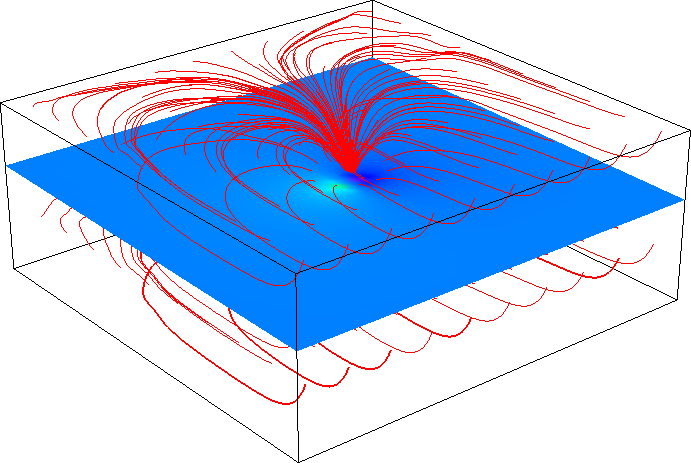
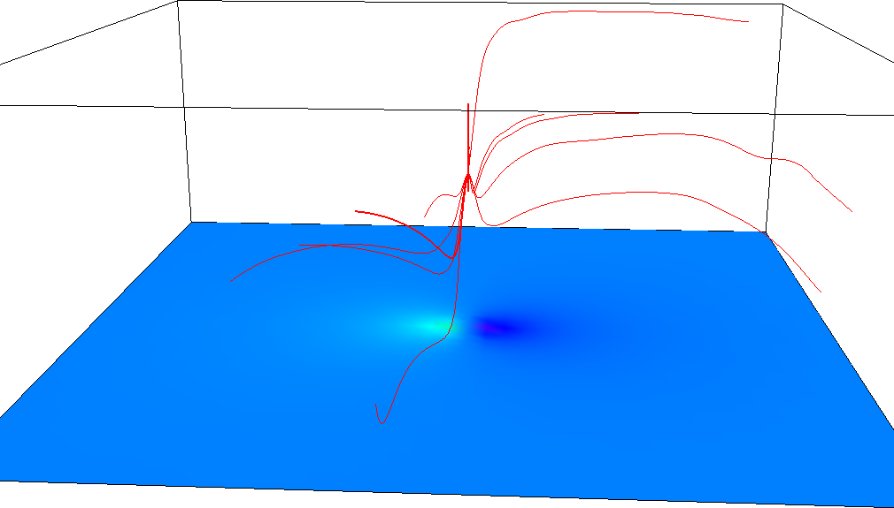
I have a running prototype producing flowlines, I tested it on artificial data created from the first example in r3.gwflow. Here are some results:

The flowlines can be generated with forward or backward integration (upstream or downstream). The integration step can be defined:

• as a time step - it is difficult to guess the right value
• as a lenght step in map units or cells (voxels) - that's now the default. The drawback is that it doesn't behave so well around singular points (where velocity is close to zero) as the time step does.

Another parameter is the maximum number of steps which prevents infinite loops I got around the singular point.

I added another input - besides the vector field components, the input can be only one 3D raster (scalar field) and I compute gradient using NumPy's method gradient.

For the next week, I would like to test it on more complicated data (space-time cube data of terrain evolution) and implement a flow accumulation analogue in 3D. I am still not sure how to proceed, I have to either ensure that the step is so small that I will have at least one point of the flowline in the intersected cell or I have to check between each two steps that I didn't skip any cells on the way.

Also I will look at implementation of Runge Kutta method with adaptive step size which might help with the flowlines near a singular point.

Week 4

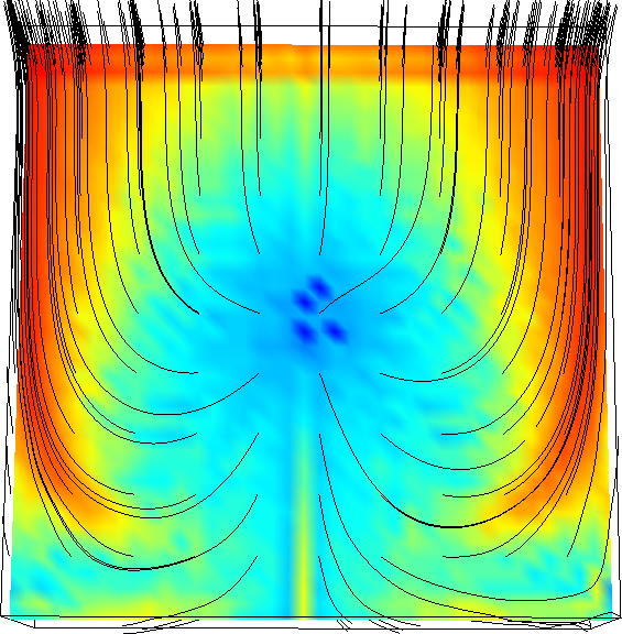
I implemented flow accumulation (number of flowlines traversing through voxel) in a naive way where I count that a flowline transects a voxel only when there is at least one point of the flowline in the voxel (cell). This doesn't work very well unless the integration step is very small. So I started to implement a voxel traversal algorithm which should say precisely which voxels are traversed (based on this ​article). I have it working now although I am not sure how to reliably test it. I will incorporate it in the flow accumulation computation.

Currently the module supports different combinations of input and output. Input can be vector map of points from which the flowlines are generated, or when not providing this vector, the flowlines are generated from centers of voxels taking into account skip parameter to reduce the number of flowlines. Output can be flowaccumulation or flowlines or both. Computation of flowaccumulation takes more time since the flowlines have to be generated from each voxel (although they are not stored in the output vector map if not specified).

Week 5

I fixed the voxel traversal algorithm and integrated in the flow accumulation computation. Computing flow accumulation works in this way: with each new point of a flowline, I test if the previous point was in the same voxel (cell) and if not I add 1 to the flow accumulation array at that particular index. Then, I check if the previous and the new point voxel index differ in more than one index (direct neighbors); if yes, I apply the traversal algorithm between these two points. This gives me indices of the possibly intersected voxels. So the flow accumulation is computed precisely comparing to a brute force approach when I would just make the integration step small enough. The voxel traversal algorithm was properly tested.

As Soeren pointed out, there will be probably some performance issues when writing to the 3D raster at random positions.

Next, I will try to implement Runge-Kutta with adaptive step size.

Week 6

I implemented Runge-Kutta with adaptive step size based on the VTK implementation and it produces satisfactory results. It is now used as default integration method.

I started to work on on-the-fly gradient computation. Gradient is computed with central differencing scheme of second order approximation (also on edges). I tested it against numpy implementation, the newest version is required because the older implementations are less precise on the edges. Then I tried to incorporate the computation of the gradient in r3.flow and it still needs some improvements and optimization. Tests show that the resulting flowlines differ slightly from flowlines computed when I use precomputed gradient. So I will look into that.

Week 7

I fixed the on-the-fly gradient computation and it gives now identical results compared to case where I use precomputed gradient arrays. The gradient array (2x2x2) is not computed every time when the algorithm requests the values, but instead, when it's close enough, it reuses the last gradient values (which happens quite often with reasonably small step size). As profiling showed, it made a significant difference. I wanted to see if computing gradient in larger window would improve it even more, however this required to rewrite this part and the code became too complicated and difficult to maintain because of handling map edges and other things that I decided to leave this approach. Moreover preliminary testing didn't show convincing improvement. I might get to it later. Then, I started rewriting the module in c, some parts which are not likely to be changed. That made me reconsider and reorganize a few things in the main script.

Week 8

I continued with rewriting the module into C and the current state is in GRASS addons (not sandbox anymore). The functionality of the module includes generating flow lines. Flow accumulation and gradient computation will follow. I tested it against the Python implementation and after fixing some problems (in both implementations) I get the same flow lines (with one type of data). The vertices along the flow lines do not match perfectly, however there is no difference in the flow lines themselves. I keep fixing the Python version, I will still use it for testing.

As expected, the C module is much much faster than the Python version. I also added function documentation.

Week 9

I rewrote the rest of the Python implementation (added flowaccumulation and on-the-fly gradient computation). I tested it against Python implementation and when computing gradient, it still differs a little bit so I will test more. Next week I will add more code documentation and try to write some tests. Also, I would like to implement integrating flowlines in both directions.

Week 10

I didn't have much time this week, so I just wrote more documentation and updated manual page with description and example. I started to write tests, I created a c test module to access the module functions and then I wrote the python test file testing interpolation. However, this broke installing the extension so I removed some changes from svn.

I also added the option to compute flowlines in both directions at once.

The differences in gradient computation from last week are resolved, it was partially caused by Rast3d_location2coord implementation, which was changed and fixed by Soeren.

Next week I would like to try different tile settings to see if there is any difference and then try to implement r3.gradient module based on the gradient function in r3.flow.